Autoscaling on Bare‑Metal: Cost‑Aware Strategies

Scaling on bare-metal servers can save costs but requires careful planning. Unlike cloud platforms with elastic scaling, bare-metal offers predictable pricing through fixed fees, avoiding charges for idle resources. However, scaling bare-metal infrastructure takes longer – up to 15 minutes – making proactive strategies crucial.
Key Takeaways:
- Why Bare-Metal?: Fixed costs, no "virtualization tax", and better control over high-performance workloads like AI.
- Challenges: Scaling isn’t instant; hardware provisioning takes time.
- Metrics to Watch: CPU, memory, GPU usage, latency (95th/99th percentile), and queue depth.
- Cost Risks: Idle resources and overprovisioning can waste 30-40% of budgets.
- Strategies:
- Use Service-Level Objectives (SLOs) to guide scaling.
- Coordinate Horizontal, Vertical, and Cluster Autoscalers.
- Apply predictive scaling with tools like machine learning to anticipate demand.
By combining metrics-driven scaling, SLOs, and predictive tools, teams can cut infrastructure costs by up to 60% while maintaining performance.
Autoscale Your on-Premises Bare Metal Kubernetes Clusters – Shukun Song, Fujitsu Limited
sbb-itb-f9e5962
Metrics That Drive Cost‑Aware Autoscaling
To make cost-aware autoscaling effective, tracking the right metrics is non-negotiable. It’s not just about CPU usage; it’s about ensuring your users get the performance they expect. Modern frameworks have shifted focus to metrics that directly reflect user experience.
Key metrics to watch include request latency (especially at the 95th and 99th percentiles), error rates, and throughput. These give you a clear picture of when your system might be falling short for users. Monitoring queue depth and request backlogs also helps you catch potential slowdowns before they impact users.
"Integrating multiple workload and system signals with explicit guardrails enables more responsive and stable scaling while preserving safety, transparency, and operator control." – Vinoth Punniyamoorthy et al.
While resource utilization is still important, it needs context. For bare-metal setups, track CPU, memory, power consumption, and cooling costs to get a full picture of expenses. For AI workloads, GPU-specific metrics like duty cycles and memory usage – captured using tools like NVIDIA DCGM Exporter – are more relevant than standard CPU metrics.
Research shows that 30% to 40% of infrastructure costs come from idle resources and overprovisioning. By adopting an SLO-driven, cost-aware autoscaling strategy, you could reduce SLO violation times by up to 31% and cut infrastructure costs by 18% compared to default Kubernetes autoscaling. Key metrics to track include time-to-scale (response speed), SLO violation duration (user impact), and replica churn (scaling stability).
Setting Service‑Level Objectives (SLOs)
SLOs set the performance limits your autoscaling must honor. Instead of asking, "Is CPU usage over 70%?" you shift to, "Are we meeting a 200ms latency target at the 95th percentile?" This changes how scaling decisions are made.
For bare-metal, provisioning new servers can take up to 15 minutes, far longer than the seconds it takes for cloud VMs. This means SLOs must allow enough buffer to manage traffic spikes while new servers come online. A common approach is setting CPU requests at 50% to 70% of observed usage and memory requests at the 95th percentile.
To fine-tune scaling, use a 7 to 14-day observation window. This accounts for weekly traffic patterns and avoids overreacting to short-term usage spikes. For latency-sensitive services, set memory limits 110% to 150% higher than requests to prevent out-of-memory errors during traffic surges.
Cost control also depends on prioritization. Using podPriorityThreshold in your cluster autoscaler ensures that new, expensive bare-metal resources are allocated only for critical workloads, not lower-priority tasks like testing. Many autoscalers scale down nodes when CPU and memory utilization drops below 50%, consolidating workloads and reducing costs.
Monitoring Resource Use and Cost Efficiency
Once SLOs are in place, monitoring becomes the backbone of smarter autoscaling. For example, CPU throttling can degrade performance, but memory overuse triggers immediate out-of-memory errors, leading to SLO violations. Keeping an eye on container_cpu_cfs_throttled_seconds_total ensures cost-saving measures don’t hurt performance.
For AI workloads, metrics like GPU queue size and batch size are better indicators of efficiency than GPU utilization alone. Over-relying on GPU utilization can lead to unnecessary scaling and wasted resources. Advanced frameworks for large language models (LLMs) have shown up to 80% reduction in GPU-hour wastage by using predictive autoscaling.
"For LLM autoscaling, GPU utilization is not an effective metric… GPU utilization tends to overprovision compared to the other metrics, making it inefficient cost wise." – Google Cloud Blog
To further optimize, clean up "zombie" containers, unused volumes, and instances with less than 30% CPU usage. Tagging resources with metadata like service, team, or environment helps identify and address cost spikes tied to specific deployments. It’s worth noting that 83% of executives see resource allocation as a key driver for growth.
Tools for Collecting and Analyzing Metrics
Tracking the right metrics requires the right tools. Here are some top options:
| Tool | Primary Function | Best For |
|---|---|---|
| Prometheus | Real-time metric collection | Kubernetes/Bare-Metal SLO tracking |
| NVIDIA DCGM Exporter | GPU telemetry (memory, temperature, health) | AI/ML workloads on bare-metal |
| KEDA | Event-driven scaling triggers | Queue-based and asynchronous workloads |
| OpenTelemetry | Multi-source telemetry aggregation | Normalizing hardware and system metrics |
| Nagios / Zabbix | Hardware and software monitoring/alerting | Bare-metal infrastructure health |
To avoid unnecessary costs during scale-down, implement protections like deletion cost management. This ensures idle or low-utilization nodes are terminated first, keeping busy nodes active during cost-cutting phases. Set cooldown periods (scaleDown.unneededTime) between 60 seconds and 10 minutes to prevent premature actions, and use a stabilization window of 300 seconds (5 minutes) to avoid frequent scaling changes.
How to Implement Cost-Aware Autoscaling on Bare‑Metal
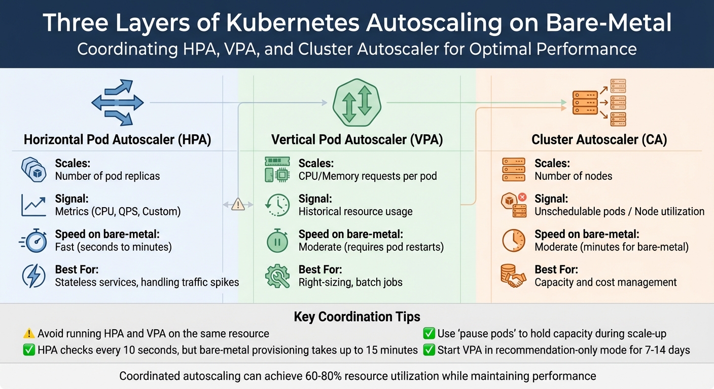
Kubernetes Autoscaling Layers Comparison: HPA vs VPA vs Cluster Autoscaler
Once you’ve nailed down the right metrics and defined your service-level objectives (SLOs), it’s time to bring cost-aware autoscaling to life. In bare-metal environments, provisioning physical servers can take up to 15 minutes. Because hardware provisioning takes longer, it’s crucial to balance immediate performance needs with careful scaling. This ensures applications stay responsive while keeping server usage in check. By optimizing Kubernetes, you can trim costs by as much as 65%. Coordinating pod-level and node-level scaling can also boost resource utilization to 60%-80% without compromising performance.
SLO-Based Autoscaling with Cost Limits
Traditional autoscaling often relies on simple thresholds like CPU usage. SLO-based autoscaling, on the other hand, focuses on meeting specific service-level goals, such as latency or throughput, ensuring that scaling decisions align with user experience.
To control costs effectively, set CPU requests at the 50th to 70th percentile of observed usage and memory requests at the 95th percentile. This strategy avoids overprovisioning while leaving room for occasional traffic spikes.
To enforce cost limits, configure the podPriorityThreshold in your Cluster Autoscaler. This ensures that new bare-metal nodes are only provisioned for high-priority workloads, skipping less critical tasks like testing or batch jobs. Autoscalers typically scale down nodes when CPU and memory usage drop below 50%, consolidating workloads to save on power and cooling costs.
"AIOps-driven, SLO-first autoscaling can significantly improve the reliability, efficiency, and operational trustworthiness of Kubernetes-based cloud platforms." – Vinoth Punniyamoorthy et al.
Another useful tool is LimitRange policies, which prevent BestEffort pods – those without defined resource requests or limits – from causing scheduling issues or unplanned evictions. These pods are often the first to be terminated under node pressure, potentially disrupting services if not managed properly.
Coordinating Pod and Node Scaling
Kubernetes autoscaling works across three layers:
- Horizontal Pod Autoscaler (HPA): Adjusts the number of pod replicas based on metrics like CPU or custom signals.
- Vertical Pod Autoscaler (VPA): Optimizes CPU and memory requests for each pod using historical data.
- Cluster Autoscaler (CA): Manages the number of nodes based on unschedulable pods or overall node usage.
To maximize efficiency, it’s essential to coordinate these layers. For example, while the HPA might add pod replicas to handle increased traffic, without the CA, those pods could remain "Pending" if the cluster lacks capacity. On bare-metal, the CA interacts with the Machine API or Cluster API to manage BareMetalHost (BMH) resources, automatically provisioning or de-provisioning nodes as needed. Keep in mind that while the autoscaler checks scaling needs every 10 seconds, provisioning a new bare-metal node can still take up to 15 minutes.
| Autoscaler | Scales | Signal | Speed (on bare‑metal) | Best For |
|---|---|---|---|---|
| HPA | Number of pod replicas | Metrics (CPU, QPS, Custom) | Fast (seconds to minutes) | Stateless services, handling traffic spikes |
| VPA | CPU/Memory requests per pod | Historical resource usage | Moderate (requires pod restarts) | Right-sizing, batch jobs |
| Cluster Autoscaler | Number of nodes | Unschedulable pods / Node utilization | Moderate (minutes for bare-metal) | Capacity and cost management |
Avoid running HPA and VPA on the same resource to prevent conflicts. A common practice is to use HPA for horizontal scaling based on custom metrics like requests per second, while VPA manages CPU and memory requests. Start with VPA in "Off" or recommendation-only mode for about a week to gather historical data before enabling automatic pod evictions for right-sizing.
To counteract the slow provisioning time of bare-metal nodes, deploy "pause pods" with very low priority. These pods hold capacity temporarily, allowing real workloads to preempt them when scaling up. This ensures immediate capacity while the CA works in the background to provision new nodes, minimizing costs during demand spikes. Additionally, ensure your Pod Disruption Budgets (PDBs) aren’t overly restrictive, as strict PDBs can block the Cluster Autoscaler from consolidating underutilized nodes.
Once these reactive strategies are in place, you can refine resource allocation further with predictive scaling.
Using Multi-Signal Forecasting
While reactive autoscaling addresses immediate needs, predictive autoscaling uses lightweight machine learning models to anticipate demand and scale resources before spikes occur. This proactive approach can improve response times by 50% and cut infrastructure costs by 40%-50%.
Multi-signal forecasting expands beyond basic CPU and memory metrics. It incorporates additional signals like requests per second (RPS), database query rates, network bandwidth, and user session counts, offering more context-aware scaling. For AI workloads on bare-metal, consider metrics like "queue size" or "batch size" to meet specific performance goals, as GPU utilization alone may not provide a full picture.
In February 2024, researchers at Sun Yat-sen University introduced BAScaler, a multi-level ML framework. It combines an Informer model for long-term predictions with an Autoregressive (AR) model for handling bursts. Tested on ten real-world workloads, BAScaler reduced SLO violations by 57% and resource costs by 10%. The system also used Deep Reinforcement Learning (PPO agent) to correct estimation errors in non-burst scenarios.
"Predictive scaling offers a proactive approach by leveraging machine learning (ML) and artificial intelligence (AI) to forecast future demand, enabling smarter resource allocation that balances cost efficiency and high availability." – Sarthak Arora, AI Research Contributor
To integrate predictive scaling, tools like KEDA can create AI-powered controllers that trigger scaling based on demand forecasts rather than current usage. Initially, run these models in recommendation-only mode – similar to VPA’s "Off" mode – to validate their predictions against real-world performance before enabling automatic scaling.
TechVZero‘s Bare‑Metal Kubernetes Autoscaling Methods
TechVZero takes a different approach to bare-metal autoscaling by focusing on predictive scaling rather than reacting to CPU spikes. Using XGBoost forecasting, the platform predicts resource demands ahead of time, avoiding over-allocation during traffic surges like DDoS attacks or CI pipeline bursts. Traditional autoscalers often overcommit resources in these situations, leading to inflated baselines. Instead, TechVZero continuously adjusts resource requests in real-time through live rightsizing. Combined with high-density bin-packing, this method boosts node utilization well beyond the typical 30%-40% seen in most Kubernetes setups. For GPU workloads, the platform dynamically allocates resources at the workload level instead of scaling entire nodes, ensuring GPUs are used efficiently. These strategies collectively deliver substantial cost savings.
How TechVZero Achieves 40%-60% Cost Savings
TechVZero’s predictive scaling doesn’t just optimize performance – it also slashes costs by 40%-60% when shifting workloads to bare-metal Kubernetes. Here’s how:
- No egress fees: By eliminating these charges, significant savings are realized.
- Optimized RI and Savings Plan usage: Resources are allocated smarter.
- Efficient handling of bursty workloads: Predictive models prevent resource overuse during unexpected spikes.
The platform’s XGBoost forecasting layer evaluates CPU, memory, and custom metrics to predict demand, avoiding resource thrashing during traffic fluctuations. This is especially useful for teams managing CI pipelines or LLM inference workloads, where traditional autoscalers often miss the mark – either lagging behind demand or wasting capacity. TechVZero’s pricing model is simple: clients pay 25% of the savings for one year, and if the platform doesn’t meet the savings threshold, clients owe nothing.
Case Study: $333,000 Saved While Stopping a DDoS Attack
A real-world example highlights the effectiveness of TechVZero’s approach. In one month, the platform saved a client $333,000 while mitigating an active DDoS attack. By leveraging XGBoost-driven predictive scaling, TechVZero distinguished between attack traffic and legitimate usage. This prevented the autoscaler from overcommitting resources, a common pitfall during such incidents. The result? Infrastructure costs were managed effectively, and Kubernetes cloud spending was reduced by 40%-70%, even under challenging conditions.
Autoscaling Setup Comparison
Here’s how TechVZero stacks up against default Kubernetes autoscaling:
| Feature | Default Kubernetes | TechVZero-Optimized |
|---|---|---|
| Scaling Trigger | Reactive (past usage) | Predictive (XGBoost forecasting) |
| Pod Rightsizing | Manual requests and limits | Live rightsizing (zero downtime) |
| Node Utilization | 30%-40% average | High-density bin-packing |
| GPU Optimization | Node-level scaling | Dynamic workload allocation |
| Cost Awareness | Basic spot/on-demand selection | RI and Savings Plan prioritization |
This comparison showcases how TechVZero transforms autoscaling into a more efficient, cost-effective process that aligns with modern workload demands. By integrating predictive analytics and smarter resource management, the platform sets a new standard for Kubernetes autoscaling.
Tools for Monitoring and Optimizing Bare‑Metal Autoscaling
To make cost-aware autoscaling effective, you need reliable monitoring tools that provide real-time insights and help keep costs in check. Prometheus is a great starting point – it collects time-series data from your bare-metal infrastructure and keeps metrics accessible even during outages. Pair this with Grafana, which transforms raw data into visual performance trends, making it easier to track autoscaling efficiency and hardware health. For cost-specific insights, OpenCost breaks down efficiency metrics like hourly costs for vCPU, GPU, and RAM at both the pod and namespace levels. Meanwhile, Telegraf gathers hardware metrics (CPU, memory, disk, and network) from bare-metal servers using the Redfish API. Additional tools like kube-state-metrics and node-exporter provide data on resource allocation and node capacity.
Real‑Time Monitoring with Open‑Source Tools
Start with Prometheus for dependable data collection – it functions independently, even during downtime. Use Grafana alongside it to visualize trends and identify optimization opportunities. For GPU-heavy workloads, track metrics such as DCGM_FI_DEV_GPU_UTIL to measure utilization and adjust workloads effectively. If you’re handling high-throughput tasks like LLM inference, queue size can serve as a useful scaling metric, helping you balance throughput and costs while staying within latency limits. To optimize data collection, set a minimum 1-minute scrape interval for cost metrics and use metric relabeling to focus on essential data like node_.* and kubecost_.*.
For larger bare-metal setups, configure Telegraf in a clustered mode with load balancing to avoid bottlenecks. Adjust the Horizontal Pod Autoscaler’s stabilization window based on workload demands – for example, set it to 0 for immediate scaling during traffic spikes, but maintain a 5-minute window for scaling down to prevent premature resource cuts. These tools not only monitor performance but also supply vital data for cost audits.
Cost Audits and Reporting
Regular cost audits are key to ensuring autoscaling aligns with your budget. These audits compare actual resource usage against allocated capacity to identify inefficiencies and cut unnecessary costs. Tools like OpenCost and Grafana calculate idle costs by analyzing the gap between actual usage and either node capacity or pod requests. Over-provisioning often shows up as discrepancies between maximum resource requests and actual usage. Use a right-size index to flag underutilized resources over a 14-day period, and track idle capacity ratios for unused vCPU, RAM, and storage. Audits can also uncover "zombie" resources, like unattached storage volumes or unused IPs, which drain funds without adding value.
To promote accountability, implement showback and chargeback models. Showback reports costs to departments, while chargeback directly bills them. Set governance thresholds, such as reviewing capacity when CPU usage exceeds 70% for seven straight days. For GPUs, review any that sit idle for over 24 hours, and require executive approval if they remain idle for more than 72 hours. Monitor egress usage and set alerts when 95th-percentile projections hit 85% of your allowance, giving you time to adjust with CDN usage or compression to avoid overages.
"Modern FinOps isn’t just about shaving costs – it’s about giving Finance, Product, and Engineering the same truth about spend, performance, and risk so they can make better decisions faster."
– OpenMetal
In bare-metal setups, customize OpenCost or Kubecost pricing sheets to reflect actual costs like hardware depreciation, power, and facilities, instead of relying on public cloud estimates. Export cost metrics to Prometheus to create custom Grafana dashboards that combine performance data with financial insights. Roll out cost governance in stages: start with inventory mapping and quick fixes (like deleting zombie volumes) in the first 30 days, move to automated alerts and egress reviews by day 60, and aim for full forecasting and tag compliance by day 90.
Conclusion
Cost‑aware autoscaling on bare‑metal infrastructure isn’t about cutting corners – it’s about matching resources to workload demands while keeping SLO performance intact. Bare‑metal servers, with their fixed‑cost structure, turn over‑provisioning into an advantage rather than a drawback. By leveraging aggressive CPU over‑subscription, teams can achieve 3‑4x compute density without the financial burden typically associated with public cloud environments.
The strategy hinges on coordinating multiple scaling layers. Horizontal and Vertical Pod Autoscalers take care of application‑level adjustments, while Cluster Autoscalers manage the hardware side. This layered approach, combined with detailed monitoring of metrics like CPU, memory, I/O, and network usage, ensures that optimizing one area doesn’t create bottlenecks elsewhere. With the average Kubernetes cluster CPU utilization sitting at just 10%, there’s a massive opportunity to improve efficiency. This multi‑layered method not only enhances resource usage but also introduces real, measurable cost control.
"The goal isn’t solely cost reduction. It’s achieving optimal resource-to-workload alignment while maintaining performance." – Keith MacKenzie, Content Marketing Manager, CloudZero
TechVZero’s workload‑centric approach tackles the 83% of compute resources that typically go unused, achieving 40‑60% cost savings through multi‑dimensional autoscaling and zero‑downtime live migration. Their performance‑based pricing model – charging 25% of savings for a year, or nothing if the target isn’t met – underscores their confidence in delivering results.
To get started, try enabling the Vertical Pod Autoscaler in recommendation mode, set namespace‑level resource quotas, and aim for 60‑80% utilization. This strikes a balance between efficient scheduling and maintaining a buffer for unexpected spikes.
FAQs
How do I pick SLO targets that work with 15-minute bare-metal scale-up times?
When defining SLO targets for scaling bare-metal infrastructure within 15 minutes, it’s important to start by profiling your workload. This helps you understand how your system responds to scaling demands and allows you to set realistic and achievable goals.
Focus on key performance metrics such as:
- Latency: How quickly the system responds during scaling.
- Throughput: The amount of data or requests handled efficiently.
- Percentiles (e.g., P99): To gauge performance consistency under load.
To manage performance dips during scaling, use error budgets. These budgets give you some flexibility to absorb minor deviations without compromising overall reliability. Additionally, implement metrics-driven scaling policies that can anticipate demand and trigger scale-up actions proactively, reducing delays.
Leveraging automated frameworks can simplify the process. These tools align your SLOs with scaling requirements while ensuring the system remains reliable and responsive under varying workloads.
Which metrics should trigger autoscaling for SaaS vs AI/GPU workloads?
For SaaS workloads, it’s essential to monitor metrics such as CPU usage, memory utilization, and request rates. These indicators help fine-tune autoscaling to meet user demand efficiently.
For AI/GPU workloads, focus on metrics like GPU utilization, token-aware metrics, KV cache performance, and batching efficiency. These factors play a key role in balancing performance with cost.
By aligning metrics with the specific needs of each workload type, you can achieve better resource allocation while keeping costs under control.
How can I prevent HPA, VPA, and Cluster Autoscaler from fighting each other?
To ensure that HPA (Horizontal Pod Autoscaler), VPA (Vertical Pod Autoscaler), and Cluster Autoscaler work together without issues, it’s important to configure each one thoughtfully. Set thresholds and constraints that reduce the chances of resource conflicts. Opt for autoscaling solutions that are designed to recognize how these mechanisms interact and adjust their behavior as needed.
Pay close attention to resource policies and limits – they play a big role in maintaining smooth operations and efficient scaling. Using integrated tools or custom configurations can help these systems coordinate better, leading to improved stability and smarter resource allocation.