Kubernetes Performance Optimization: Best Practices

Kubernetes is powerful, but it’s easy to waste resources or face performance issues without proper management. Here’s what you need to know:
- Overprovisioning is costly: 70% of organizations overspend due to allocating more resources than needed.
- Scaling inefficiencies: Misconfigured autoscalers or ignoring short-term spikes can lead to underutilized resources or instability.
- Resource mismanagement: Incorrect CPU/memory limits cause throttling, latency spikes, or crashes.
Key Takeaways:
- Set accurate resource requests/limits using real usage data to avoid waste or resource contention.
- Balance workloads across nodes to maximize efficiency and prevent bottlenecks.
- Improve pod scheduling with tools like node affinity, taints, and topology spread constraints for better placement.
- Use autoscalers wisely: Horizontal Pod Autoscaler (HPA) adjusts pod replicas; Vertical Pod Autoscaler (VPA) tweaks resource allocations.
- Monitor metrics: Focus on CPU/memory usage, pod availability, and node health to identify and fix issues early.
Switching to bare metal Kubernetes can also cut costs by 40-60%, eliminating cloud overhead and improving hardware utilization. Start by analyzing usage patterns, fine-tuning autoscalers, and leveraging advanced monitoring tools like Prometheus.
Want to save money and boost performance? These strategies can help you take control of your Kubernetes setup.
Kubernetes Performance Tuning Workshop | Anton Weiss
Resource Allocation Best Practices
Proper resource allocation is the backbone of Kubernetes performance. The Kubernetes scheduler uses resource requests to determine the best placement for your pods, ensuring they fit within the available capacity of a node. At the same time, resource limits act as strict boundaries, enforced at the container level, to prevent overuse. By basing these values on actual usage data rather than rough estimates, you can avoid wasting resources or causing performance bottlenecks.
Setting Resource Requests and Limits
To set accurate resource requests and limits, start by gathering real usage data with commands like kubectl top pod and kubectl top node. Kubernetes measures CPU in units, where 1 CPU equals one physical or virtual core, with precision down to 1m (0.001 CPU). Memory is measured in bytes but is typically represented using suffixes like Mi (mebibytes) or Gi (gibibytes). For example, 129M translates to approximately 123Mi.
CPU and memory limits function differently when exceeded. If a container hits its CPU limit, the kernel throttles it using the Completely Fair Scheduler (CFS) quota, which increases latency but doesn’t terminate the container. On the other hand, exceeding a memory limit causes the container to terminate with an OOMKilled status, often with exit code 137. Because of this, it’s wise to set memory limits more conservatively than CPU limits.
As of Kubernetes v1.34, you can define pod-level resource specifications, allowing you to set an overall resource budget for a pod rather than configuring each container individually. This approach enables containers within the same pod to share unused resources, simplifying resource management and improving efficiency. Additionally, Kubernetes v1.35 introduced in-place resizing, letting you adjust CPU and memory requests and limits for running containers without recreating the pod. To enable seamless CPU scaling, set restartPolicy: NotRequired. For memory adjustments, consider using RestartContainer if your application cannot dynamically manage its heap.
Once resource requests are set, the next step is to ensure efficient distribution of workloads across nodes.
Balancing Resource Use Across Nodes
Accurate resource requests are essential, but balancing workloads across nodes is equally critical for maximizing cluster efficiency. The Kubernetes scheduler bases pod placement on requested resources, not actual usage. This means nodes may reject new pods even if they appear underutilized, simply because the sum of all requests exceeds their capacity. Using larger nodes, such as 4xlarge to 12xlarge instances, can help reduce the percentage of resources reserved for system overhead, leaving more room for pods. As highlighted in Amazon EKS Best Practices:
Using node sizes that are slightly larger (4-12xlarge) increases the available space that we have for running pods due to the fact it reduces the percentage of the node used for ‘overhead’ such as DaemonSets and Reserves for system components.
Monitor saturation in addition to utilization. A node can be fully utilized but not saturated if no tasks are waiting for resources. Use PSI (Pressure Stall Information) metrics to identify contention in CPU, memory, or I/O, which provides a clearer picture of potential bottlenecks. To prevent any single team from consuming excessive resources, implement ResourceQuota objects at the namespace level. If pods get stuck in a Pending state with a FailedScheduling event, use kubectl describe nodes to determine whether the requested resources exceed the node’s allocatable capacity.
Improving Pod Scheduling
After setting resource requests and balancing workloads across nodes, the next step is managing where pods are placed. While Kubernetes’ default scheduler bases placement on available resources, it doesn’t consider hardware needs, network proximity, or failure domain distribution. By leveraging node affinity, taints and tolerations, and topology spread constraints, you can fine-tune pod placement for better performance and reliability.
Using Node Affinity and Taints/Tolerations
Node affinity allows you to control pod placement using node labels. It’s more flexible than nodeSelector, offering two types of rules: requiredDuringSchedulingIgnoredDuringExecution for strict requirements and preferredDuringSchedulingIgnoredDuringExecution for softer preferences. For instance, you can specify that a pod must run on nodes with SSDs (hard rule) or prefer SSD nodes but allow fallback to standard disks (soft rule).
Start with soft preferences to observe scheduler behavior before applying stricter rules. You can also use a topologyKey (like kubernetes.io/hostname) to define the scope for pod placement.
To colocate services that frequently communicate, use inter-pod affinity. For example, a web application and its cache layer perform better when placed on the same node. On the other hand, anti-affinity helps spread replicas across nodes or failure domains, ensuring that a single node failure doesn’t take down the entire application. However, keep in mind that inter-pod affinity and anti-affinity can slow down scheduling in clusters with hundreds of nodes.
Taints and tolerations complement affinity by preventing pods from running on unsuitable nodes. Taints are applied to nodes, signaling that only specific pods can tolerate them. Tolerations are added to pods, allowing them to "accept" certain taints.
| Taint Effect | On Scheduling | On Eviction | Use Case |
|---|---|---|---|
| NoSchedule | Blocks new pods | None | Reserving nodes for specific workloads |
| PreferNoSchedule | Avoids placing new pods | None | Steering pods away from busy or costly nodes |
| NoExecute | Blocks new pods | Evicts non-tolerating pods | Draining nodes for maintenance or failures |
For specialized hardware like GPUs, use taints to repel general-purpose workloads and node affinity to attract specific ones. To ensure exclusivity, combine taints with node labels and corresponding affinity rules. For applications with large local states, set tolerationSeconds with the NoExecute taint to delay eviction (e.g., 3,600 seconds), giving the node time to recover and avoid unnecessary disruptions.
You can further refine pod distribution with topology spread constraints.
Implementing Topology Spread Constraints
Topology spread constraints offer a detailed way to distribute pods across failure domains such as zones, regions, or nodes. Unlike pod anti-affinity, these constraints focus on maintaining balanced distribution ratios rather than strict placement rules. This prevents resource contention and performance issues caused by too many pods concentrating on a single node.
The main parameters are:
maxSkew: Defines the maximum difference in pod count between any two domains. For example, amaxSkewof 1 ensures the difference between domains doesn’t exceed one pod.topologyKey: Specifies the domain for distribution, such askubernetes.io/hostnamefor nodes ortopology.kubernetes.io/zonefor zones.whenUnsatisfiable: Determines the scheduler’s behavior if constraints can’t be met. Options includeDoNotSchedule(hard rule) orScheduleAnyway(soft rule that minimizes skew).
For smaller deployments (2-3 replicas), pod anti-affinity may suffice. But for larger workloads (4+ replicas), topology spread constraints are more effective. For critical applications, consider nested constraints: use a strict maxSkew for zones to ensure resilience and a softer maxSkew for nodes to maintain flexibility. Be cautious with hard constraints like DoNotSchedule in small clusters, as they can leave pods stuck in a "Pending" state if the conditions aren’t met.
Pair topology spread constraints with the Horizontal Pod Autoscaler (HPA) to ensure that as your application scales, new replicas are evenly distributed across your infrastructure.
Scaling Kubernetes Clusters
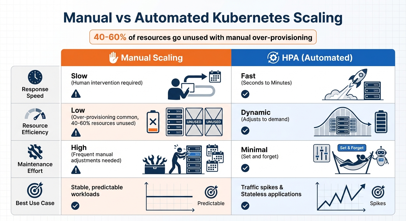
Manual vs Automated Kubernetes Scaling: Performance and Efficiency Comparison
Once you’ve optimized pod placement, the next step is setting up scaling to handle fluctuating workloads. Kubernetes provides two main scaling approaches: horizontal scaling, which adds or removes pods, and vertical scaling, which adjusts the resources allocated to pods. Both methods need careful configuration to ensure resources aren’t wasted or users aren’t left waiting during traffic spikes. When done right, scaling keeps your cluster responsive and efficient.
Configuring the Horizontal Pod Autoscaler
The Horizontal Pod Autoscaler (HPA) dynamically adjusts the number of pod replicas based on metrics like CPU usage, memory consumption, or custom signals. The formula it uses to determine the number of replicas is:
desiredReplicas = ceil(currentReplicas * (currentMetricValue / desiredMetricValue))
HPA evaluates metrics every 15 seconds and only acts when the change exceeds a 10% tolerance threshold.
Before enabling HPA, make sure to remove the spec.replicas field from your Deployment manifests. If this field remains, running kubectl apply could reset the replica count, causing conflicts between the manifest value and HPA’s calculated number. Also, ensure you’ve defined resource requests (refer to Resource Allocation Best Practices).
To prevent rapid fluctuations in scaling, HPA uses a stabilization window. By default, the scale-down window is set to 5 minutes, meaning it considers the highest recommendation from the last 300 seconds before reducing replicas. You can customize this behavior through the behavior field in the autoscaling/v2 API. For example, you might limit scale-down actions to 10% of pods per minute.
For specific workloads like API gateways or message processors, where CPU usage doesn’t directly reflect demand, you can configure HPA to use custom metrics, such as requests-per-second or queue length, instead of CPU percentages. If your pods include sidecars that create resource spikes, configure HPA to focus on metrics for the main application container and ignore the sidecar’s usage. Additionally, pair HPA with Pod Disruption Budgets (PDBs) to ensure a minimum number of pods remain available during scale-down events. Together, these configurations help maintain performance while optimizing resource use.
Manual Scaling vs. Automated Scaling
Manual scaling may seem straightforward, but it’s often slow and requires constant attention. During demand surges, you might find yourself adding replicas manually or over-provisioning to avoid downtime, which can result in 40% to 60% of resources going unused.
Automated scaling with HPA, on the other hand, reacts to changes in demand within seconds or minutes. However, it requires fine-tuning of stabilization windows and thresholds to avoid instability. Comparing the two approaches highlights their distinct advantages and limitations:
| Feature | Manual Scaling | HPA (Automated) |
|---|---|---|
| Response Speed | Slow (Human intervention) | Fast (Seconds/Minutes) |
| Resource Efficiency | Low (Over-provisioning) | Dynamic |
| Maintenance Effort | High (Frequent adjustments) | Minimal |
| Best Use Case | Stable, predictable loads | Traffic spikes/Stateless apps |
If you combine HPA with the Vertical Pod Autoscaler (VPA), avoid configuring both to act on the same metric. For instance, let HPA scale based on a custom metric like requests-per-second while VPA manages memory adjustments. If both must operate on the same resource, configure HPA to use averageValue (absolute usage) instead of averageUtilization (percentage) to prevent feedback loops where VPA’s adjustments trigger unnecessary scaling actions.
Start with VPA in "Recommendation" mode to review its suggestions for resource adjustments before enabling full automation. Set minAllowed and maxAllowed resource policies to keep scaling within budget and capacity limits. For applications with long startup times, such as Java-based workloads, configure startupProbes with an initialDelaySeconds value that accounts for the high CPU usage during initialization. This ensures HPA doesn’t misinterpret startup spikes as a need to scale up unnecessarily.
sbb-itb-f9e5962
Monitoring and Troubleshooting Performance
Keeping a close eye on your Kubernetes cluster is essential for catching performance issues before they snowball into bigger problems. Without proper monitoring, things like CPU throttling can sneak up on you, causing unexpected latency spikes and leaving you scrambling to find the root cause. Itiel Shwartz, Co-Founder and CTO at Komodor, highlights the risk:
It is very dangerous to be CPU throttled without being aware of it. Latencies of random flows in the system spike up and it might be very hard to pinpoint the root cause.
Kubernetes offers two main metric pipelines to help you monitor your cluster. The Resource Metrics Pipeline (via metrics-server) powers tools like kubectl top and the Horizontal Pod Autoscaler, while the Full Metrics Pipeline (typically Prometheus paired with Grafana) provides deeper insights, including long-term trends and custom metrics. To get even more detailed data, deploy kube-state-metrics alongside Prometheus. This setup adds information about Kubernetes objects, like deployment replicas and pod statuses. If you’re running Linux kernel 4.20 or newer with cgroup v2, enabling PSI metrics can help you track resource wait times at the node, pod, or container level.
Key Metrics to Track
Certain metrics are vital for ensuring a smooth user experience and maintaining cluster stability. For instance, resource usage should generally stay between 60% and 80% of requested resources at the 90th percentile. If actual usage is much lower than requests, you’re likely overspending. On the flip side, if usage exceeds requests, you risk resource contention. Keep a close eye on container_cpu_usage_seconds_total and container_memory_working_set_bytes. Exceeding CPU limits can lead to throttling and latency spikes, while breaching memory limits can result in OOM (Out of Memory) kills.
Pod availability is another critical area to monitor. Look at the percentage of unavailable pods compared to desired replicas to identify issues like "Pending" states (caused by insufficient resources) or "CrashLoopBackOff" errors (linked to application problems or resource limits). Additionally, track scheduler_pod_scheduling_attempts; high numbers here might indicate resource shortages or conflicts with affinity rules.
When it comes to node health, focus on the "Ready" status and watch for pressure indicators such as DiskPressure, MemoryPressure, and PIDPressure. These signals show when a node is struggling to host workloads safely. If a node reports "Ready=False" or any pressure condition turns "True", act immediately.
For control plane stability, monitor metrics like apiserver_request_duration_seconds. High latency here can slow down kubectl commands and disrupt controller operations. In terms of storage, keep an eye on kubelet_volume_stats_used_bytes and set up systems to forecast storage needs. Ideally, you should have a two-to-three-week buffer before Persistent Volumes fill up, as full volumes can cause write failures and crashes.
Tracking these metrics is the first step. The next is setting up alerts to catch problems before they escalate.
Setting Up Alerts for Critical Issues
Alerts should focus on sustained conditions to avoid unnecessary noise. For example, set alerts for 80% of CPU limits sustained over five minutes and 90%-95% of memory limits sustained for one to two minutes. To catch sudden changes, use Prometheus’s rate() function. For instance, alert if CPU usage spikes by 30% within five minutes, as this often signals an impending crash.
If you’re using Horizontal Pod Autoscalers (HPA), set alerts for when desired replicas hit 85% of the maximum. This gives you time to scale up manually or adjust your infrastructure. Also, monitor container restart rates – frequent restarts often point to deeper configuration or resource issues. Use Alertmanager to group related alerts and send them to channels like Slack or PagerDuty based on severity.
The Prometheus project offers wise advice:
Aim to have as few alerts as possible, by alerting on symptoms that are associated with end-user pain rather than trying to catch every possible way that pain could be caused.
Don’t forget to monitor the monitoring tools themselves. If Prometheus or Alertmanager goes offline, you need to know right away. For workloads with variable traffic patterns, consider using dynamic thresholds with PromQL. These adjust based on historical data, making your alerts more accurate. Establish baselines by collecting historical data to define "normal" operating ranges for your workloads, which helps improve anomaly detection.
Cost Optimization with Bare Metal Kubernetes
While earlier discussions highlighted performance and scaling, tackling cost inefficiencies is equally important. Running Kubernetes in the cloud often comes with a hefty "cloud tax", driven by overprovisioning, managed service fees, and virtualization overhead. These factors can inflate costs by as much as 30–60%. For instance, cloud providers typically charge $200–$500 per node per month, yet average CPU utilization remains a meager 12–18%, exposing a significant gap in efficiency.
Cloud schedulers, designed to distribute pods across nodes for resilience, often leave many machines underutilized – operating at just 20–40% efficiency. Bare metal environments, on the other hand, avoid the resource fragmentation that plagues virtualized setups. Additional expenses, such as $16 monthly fees for Application Load Balancers and control plane management costs, further compound these inefficiencies. These challenges make a strong case for exploring alternative solutions like bare metal Kubernetes, as demonstrated in a real-world migration example.
Case Study: Cutting Costs by 40–60% with Bare Metal
TechVZero successfully migrated a client to bare metal Kubernetes, slashing costs by $333,000 in just one month. By eliminating virtualization overhead and managed service fees, the client achieved a remarkable 40–60% reduction in total costs. This case underscores how bare metal can deliver both financial savings and reliable performance under demanding conditions.
Bare metal environments remove inefficiencies by granting direct access to hardware. Unlike virtual machines – where hypervisors add unnecessary overhead and nodes are deemed "full" based on requested rather than actual usage – bare metal allows for tighter bin packing and higher utilization rates. For example, a financial services firm running nightly ETL jobs uncovered they were overprovisioning by 85% (requesting 8 CPU cores and 32 GB of RAM while only using 1.2 cores and 4 GB). By adjusting their resource allocation, they saved $180,000 annually.
Performance and Cost Advantages of Bare Metal
The benefits of bare metal go beyond just cutting costs; it also delivers superior performance. Bare metal Kubernetes provides unparalleled control over hardware, enabling precise CPU isolation for performance-critical workloads. It also supports features like hugepages (1 GiB or 2 MiB) for memory-intensive applications and NUMA awareness, ensuring CPU-bound applications get dedicated access without interference. These optimizations, often unachievable in virtualized environments, directly contribute to cost efficiency.
One example of this is a multi-tenant SaaS provider that consolidated node groups and optimized DaemonSet allocation. This adjustment reduced their monthly compute costs from $70,070 to just $5,337 – a staggering 92% savings – while still meeting all service-level objectives. Additionally, workloads such as JVM-based services or large language models, which often struggle with cold starts and virtualization overhead, benefit significantly from bare metal’s ability to eliminate these bottlenecks.
With bare metal, the billing model shifts from unpredictable per-node charges to fixed capital expenditures or hardware leases. This transition not only makes costs more predictable but also simplifies infrastructure planning, offering businesses a clearer path to long-term scalability and efficiency.
Conclusion
Kubernetes optimization plays a key role in ensuring efficient scaling and keeping costs under control. By accurately setting resource requests and limits, you can avoid "OOMKilled" crashes and resource contention. Implementing Horizontal Pod Autoscaling (HPA) ensures that capacity aligns with real-time demand. Additionally, smart pod placement strategies, like using node affinity and taints/tolerations, help avoid bottlenecks – especially crucial for SaaS companies managing traffic surges or AI workloads that require GPU-enabled hardware.
A common challenge organizations face is overspending due to overprovisioning and inefficient resource use. Moving beyond basic utilization metrics and focusing on advanced monitoring, like Pressure Stall Information, can reveal hidden bottlenecks that averages often obscure. As highlighted in Amazon EKS Best Practices:
The more performant the application and nodes are, the less that you need to scale, which in turn lowers your costs.
By applying the strategies outlined here – focused on resource management, scaling, and monitoring – you can set the foundation for practical next steps.
Next Steps for Kubernetes Optimization
Start by capturing workload patterns over 7–14 days using tools like kubectl top and Prometheus. Reduce container image sizes by 60–80% with multi-stage Docker builds to speed up pod startup times. Deploy the Vertical Pod Autoscaler (VPA) in recommendation mode, and analyze its suggestions for at least 24 hours before enabling automatic updates. Use Pod Disruption Budgets (PDBs) to ensure minimum availability during node maintenance or upgrades. For large clusters, adjust the scheduler’s percentageOfNodesToScore setting to strike a balance between scheduling speed and placement precision.
Getting Results with TechVZero

Executing these best practices is where TechVZero shines. TechVZero specializes in optimizing Kubernetes for engineering-focused founders, allowing them to concentrate on product development. With experience managing over 99,000 nodes, we’ve helped clients achieve remarkable results – like saving $333,000 in just one month while mitigating a DDoS attack during the same engagement. Our bare metal Kubernetes migrations typically reduce costs by 40–60% compared to managed cloud services, delivering the same reliability at a fraction of the price.
What sets us apart? Our performance-driven model: we charge 25% of the savings for one year, with no fees if targets aren’t met. Whether you require SOC2, HIPAA, or ISO compliance, we offer comprehensive infrastructure solutions tailored for teams of 10–50 people. Visit TechVZero to learn how we can optimize your Kubernetes infrastructure and help you achieve your goals.
FAQs
How do I set accurate resource requests and limits in Kubernetes?
To configure accurate resource requests and limits in Kubernetes, the first step is to measure how much CPU and memory your application actually uses. Run your workload without any predefined limits, and use tools like metrics-server or Prometheus to monitor its resource consumption. A good rule of thumb is to use the 95th-percentile values as your starting point.
For requests, set the minimum resources your application needs to operate reliably. For instance:
resources: requests: cpu: "0.5" # Reserves 0.5 CPU core memory: "256Mi" # Reserves 256 MiB of RAM For limits, set values slightly higher than the requests to allow for occasional spikes while avoiding excessive resource usage:
resources: limits: cpu: "1" # Maximum of 1 CPU core memory: "512Mi" # Maximum of 512 MiB of RAM After defining these values, apply the configuration using kubectl apply -f <file>.yaml. Once deployed, keep an eye on your pods to ensure they aren’t being throttled for CPU or terminated due to running out of memory. If issues arise, tweak the values to strike a balance between performance and efficient resource usage.
To make this process even smoother, consider integrating resource tuning into your CI/CD pipeline. Automating this for new container images can help maintain cluster stability and keep operational costs in check.
What are the advantages of using bare-metal Kubernetes instead of cloud-based services?
Bare-metal Kubernetes gives you direct access to physical hardware, skipping the hypervisor layer entirely. The result? Lower latency and higher performance – a perfect match for workloads that demand intense CPU power or are highly sensitive to latency. On top of that, it lets you fine-tune optimizations, like tweaking network settings, configuring storage, or using CPU pinning. These adjustments can significantly boost efficiency, especially when you’re scaling up or working with specialized hardware.
But it’s not just about performance. Bare-metal setups also provide enhanced security and control. Since the hardware isn’t shared with other users, you can implement stricter isolation measures, roll out custom firmware updates, and avoid issues like the "noisy neighbor" effect that often plagues multi-tenant cloud environments. Plus, it can be easier on your budget – no per-CPU-hour pricing or over-provisioning to compensate for virtualization overhead.
At TechVZero, we’ve seen how bare-metal Kubernetes can deliver exceptional results in terms of performance, security, and cost savings. It’s an excellent choice for founders and engineers who want maximum control without unnecessary layers of complexity.
What are topology spread constraints, and how do they enhance pod distribution in Kubernetes?
In Kubernetes, topology spread constraints let you manage how Pods are spread across various failure domains, such as zones, nodes, or custom-defined topology keys. By distributing Pods more evenly, these constraints contribute to better availability, lower latency, reduced network costs, and improved resource usage.
This setup allows workloads to be more resilient against failures while maintaining performance efficiency. It’s an essential method for ensuring scalability and reliability in Kubernetes deployments.